Faster Trajectory Clustering using cluster2

Before proceeding in this section, one should be familiar with the trajectory clustering discussion and procedures supplied with each HYSPLIT distribution. The faster cluster2 program clusters HYSPLIT formatted trajectory files using the same input and output files as the HYSPLIT clustering method. The cluster2 program generates the CLUSLIST_{nc} output file directly for a predetermined number of clusters (nc), thereby not requiring the cluslist program. The CLUSLIST_{nc} file is then read by clusmem to create a file of trajectory file name listings for each cluster member (#} and written to the file CLUSTRAJ{#}_{nc}. This file is then read by trajmean to create a mean HYSPLIT formatted trajectory file for each cluster member number and named C{#}mean.tdump. These file names are accumulated in file MEAN.LIST which is then read by merglist to create the final cluster mean trajectory file Cmean.tdump. The mean trajectory can then be displayed using the conventional plotting program trajplot.

• Program Details for cluster2
  

  The clustering computation works in a manner similar to the clustering program distributed with HYSPLIT. Trajectories or mean clusters are merged together if that pair has the minimum spatial variance compared to all other pairs. The main improvement is that cluster2 uses a first-guess solution to permit a faster convergence rather than starting with each trajectory in its own cluster. Initially all trajectories are assigned to a first-guess cluster. Unlike the standard clustering program, the final number of clusters desired has to be preset on the command line (-n option). The program is fast enough that multiple solutions can easily be computed. Note that the percent change in total spatial variance with each clustering step is not produced by this program, thereby eliminating the need for clusplot. The remaining programs in the HYSPLIT distribution: clusmem, trajmean, merglist, and trajplot, are used to create the final graphic. The program is written in Fortran and needs to be compiled and the executable placed in the hysplit/exec directory. A sample script to run the clustering and create the graphics is provided.

• Comparing cluster and cluster2 with Testing Data
  

  In the standard HYSPLIT distribution, the testing directory contains a script (xcluster_example_svg.scr) to cluster the existing trajectories in the hysplit/cluster directory. This script has been modified and called xcluster2_example_svg.scr which will cluster the same trajectories using the faster cluster2 program. The $PGM/cluster in the script was replaced with $PGM/cluster2 -iINFILE -n3 and the calls to clusplot, clusend, cluslist, and any file existence tests that might cause the script to fail were commented out. The resulting mean clusters for the original clustering program are shown on the left and the results from the new cluster2 program on the right. A cursory view suggests they are very similar, but there are some substantial differences in the frequency of the three different clusters.

  Standard Cluster	Faster Cluster2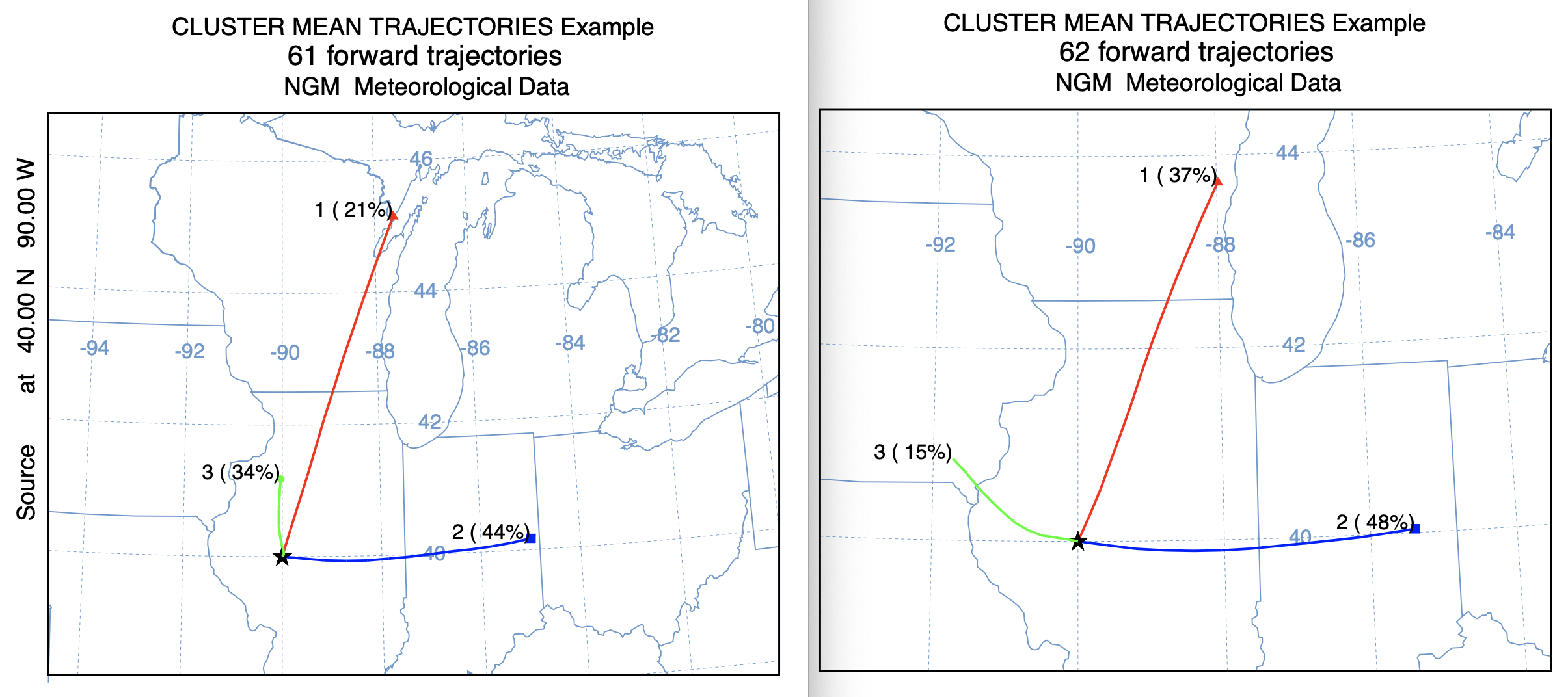

  


• Comparing Trajectories within Each Cluster
  

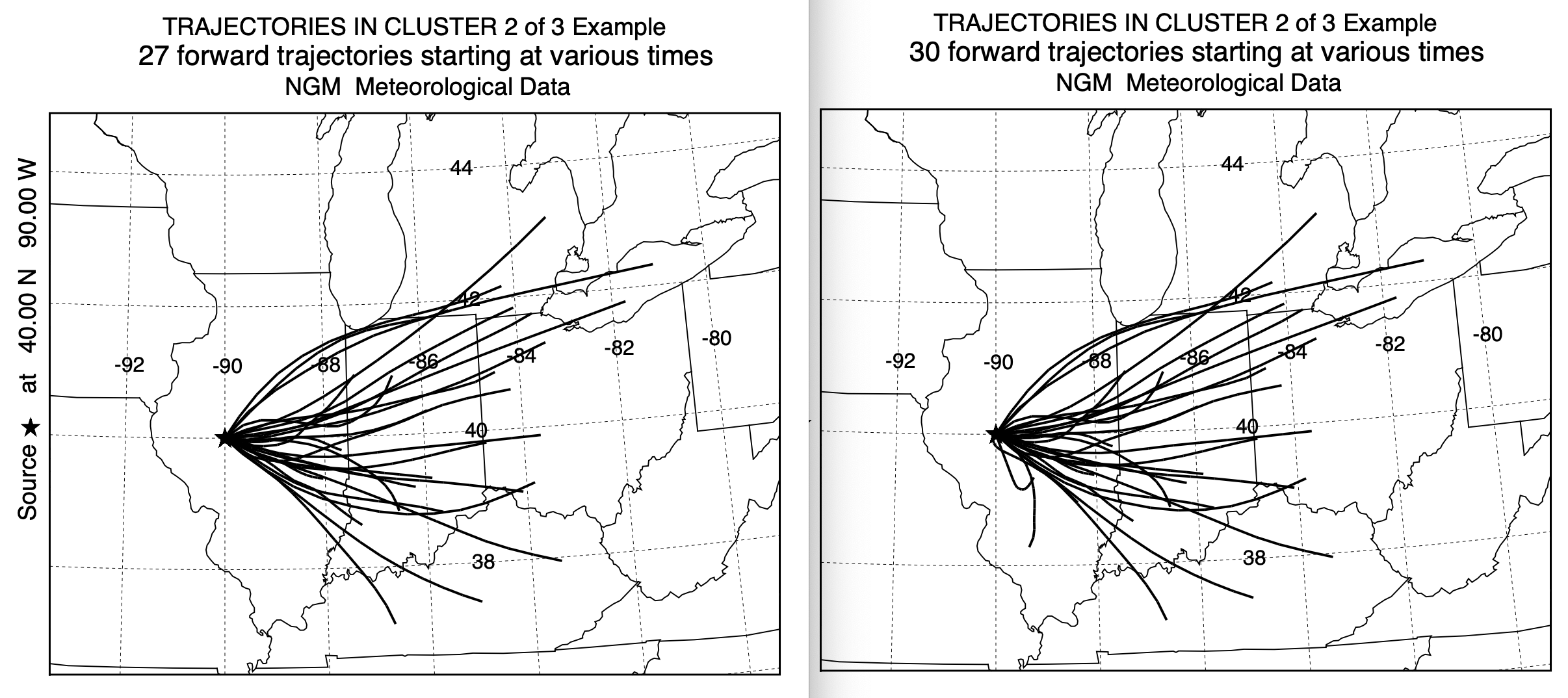
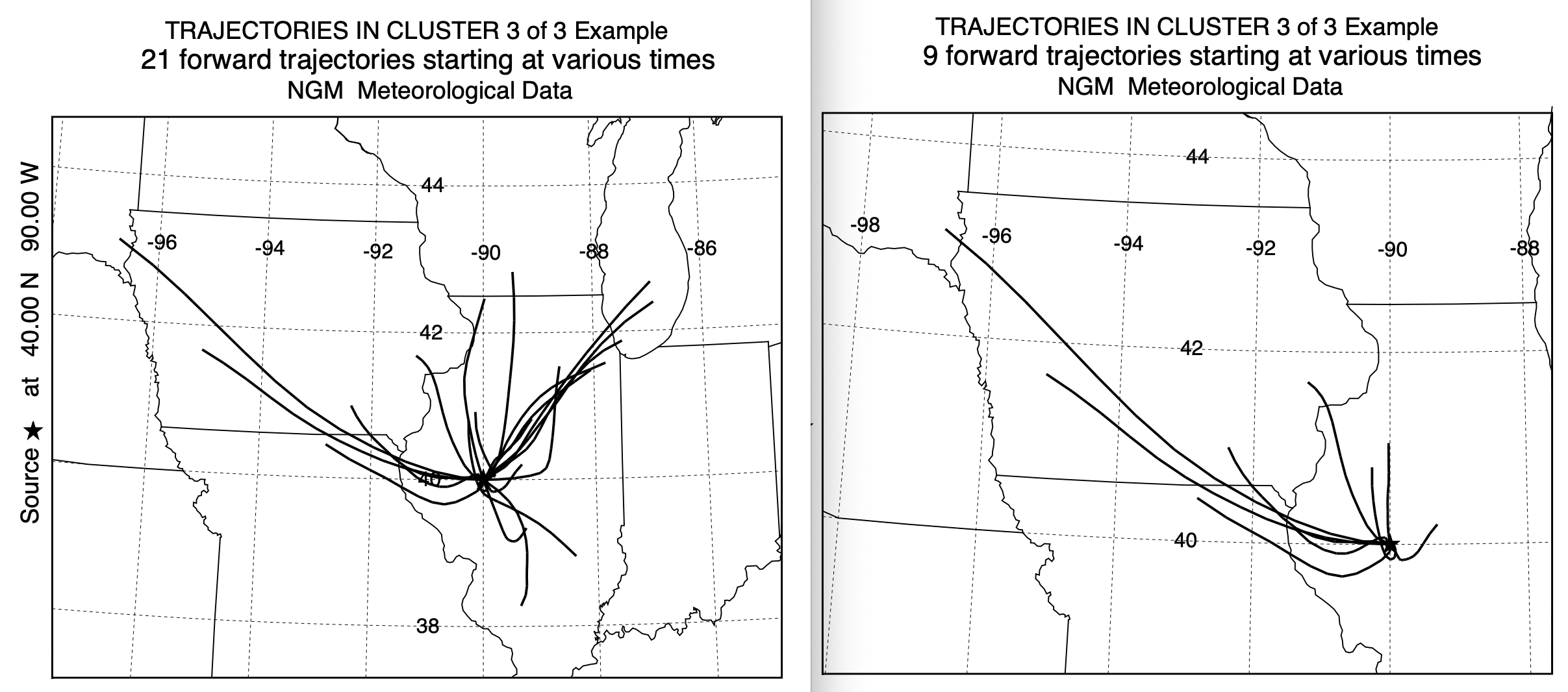
  With a 3-cluster result it is easy to examine the individual trajectories composing each cluster mean. In this case, as shown below, original on the left, new on the right, the trajectories within clusters 1 and 2 have very similar characteristics. However, in cluster number 3, the standard clustering approach contained trajectories toward the northeast, that clearly belonged in cluster 1 or 2. This accounts for the larger percentage of trajectories in cluster 1 when using the new cluster2 program. The results in this test case seem to be more favorable toward using the newer program, it may not hold true in other situations. However, there is another factor to consider - computational time.

  Standard Cluster	Faster Cluster2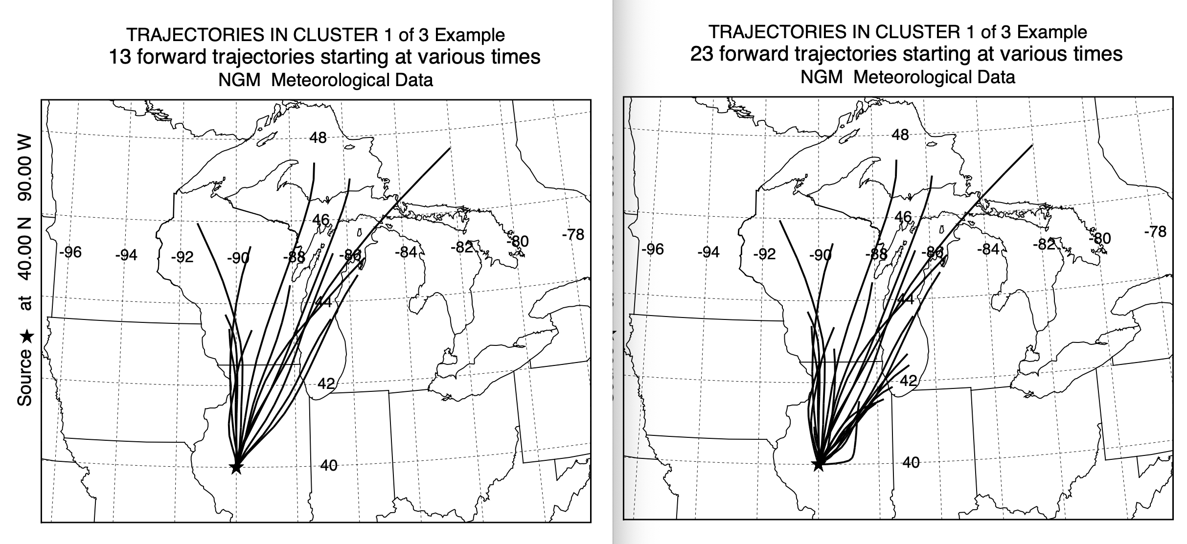

  
  
  
  


• Computational Times for Clustering
  

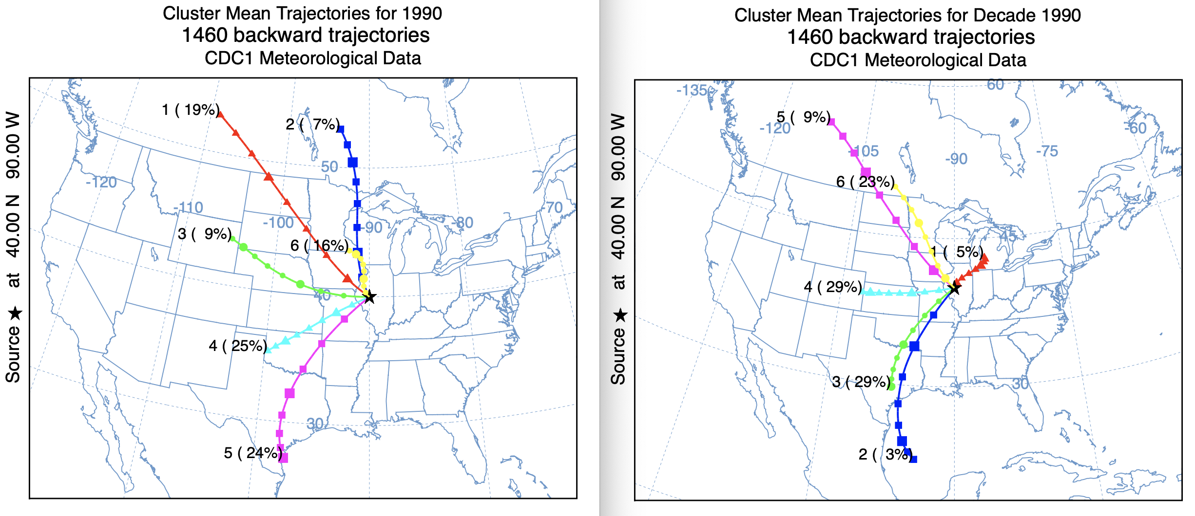
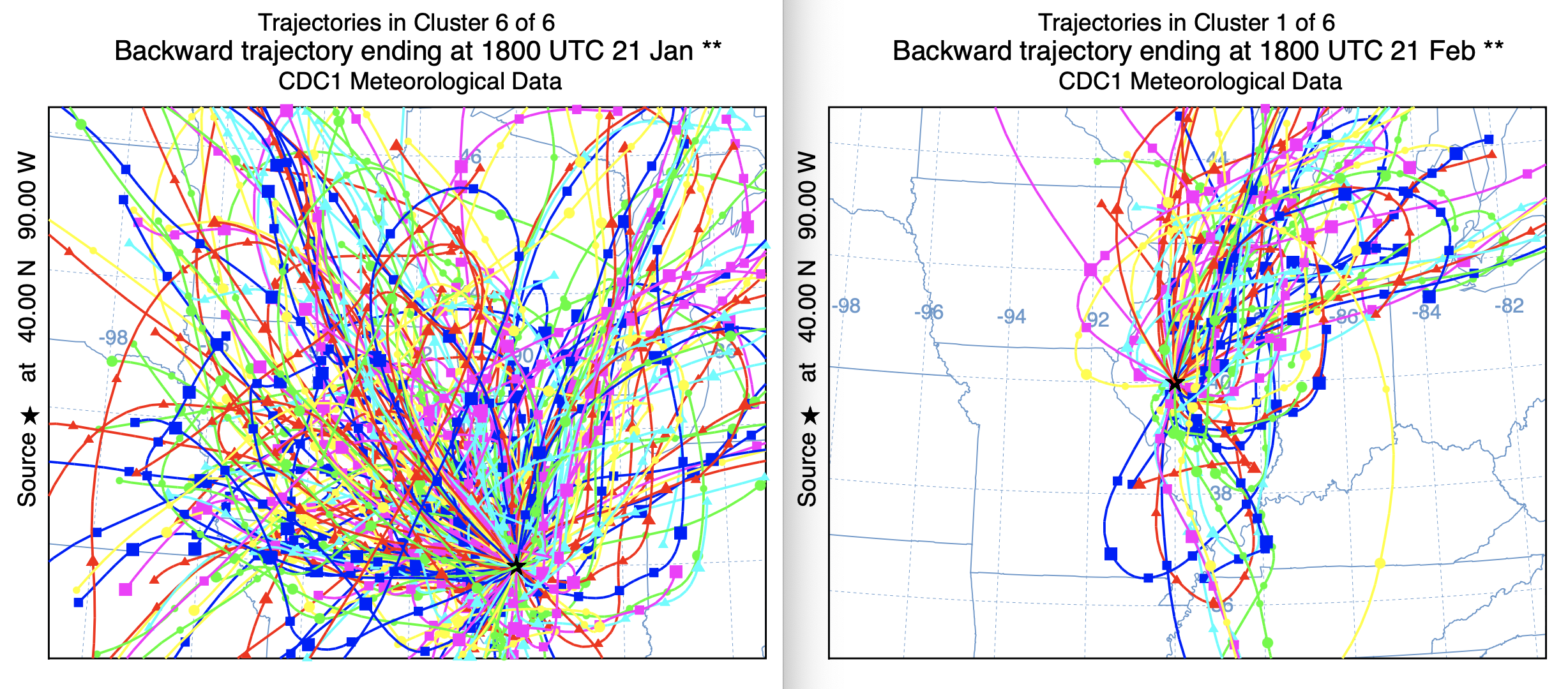
  The primary motivation to develop a new clustering approach was the computational time issue associated with clustering multiple years of trajectories. The standard approach was too prohibitive, restricting computations to a few years at best. A simple test was constructed by computing 48-h back trajectories four times a day for the year 1990. A script was used to run the original cluster and new cluster2 programs. A date command within the script, before and after the clustering showed that the standard program took about 8 minutes while the new cluster2 program took about 20 seconds. The new approach makes clustering large data sets possible. A comparison of the cluster mean trajectories shows some differences, but not as dramatic as might seem due to the differences in the projection scale. One interesting difference is cluster 1 in the new version compared with cluster 6 in the standard version, which seems to contain many more westerly directed trajectories not evident in the new approach and which would account for the direction shift between the mean trajectories for cluster 6 and cluster 1. This result has similarities to the previous result from the testing directory, where it appears that the newer approach has more skill is discerning different flow regimes when winds are light and variable or rapidly changing with time.

  Standard Cluster	Faster Cluster2

  
  
  


• Version 3 of the Fast Clustering
  

  If less dependence upon the intermediate clustering programs in the standard HYSPLIT distribution is desired, then a revision of cluster2 called cluster3 was developed which is almost identical to cluster2 but it also creates the final Cmean.tdump file. Therefore, none of the intermediate program steps are required and the clustering results can be plotted directly using trajplot. A sample script is provided and it runs slightly slower than cluster2 due to the additional processing required to create the cluster mean trajectories.

An example of what can be accomplished with a faster clustering program is presented as a decadal climate analysis. Forty eight hour back trajectories were computed using global meteorological data, 4 times per day, for 612 locations around the world, for 75 years from 1950 through 2024. Approximately 15,000 trajectories per location per decade were clustered to evaluate if any climate trends were evident in the clusters.