A Global Transport Model for Krypton-85   

This page describes a global scale modeling method that was used to subtract the time-varying background concentration of krypton-85 from a series of measurements that were made in the United States during the 1970s and 1980s. After removing the background concentrations, the resulting data represent the plumes from the nearby emission sources and then could be used for transport and dispersion model evaluations. The background subtraction methodology, but not the computer code, was published¹ earlier. More detailed information about the use of the global model as well as links to the souce code are provided in this section.

• The HYSPLIT code includes an embedded global Eulerian model (GEM) for transport and dispersion. Although the application of GEM is not discussed in any of the training materials, it can be configured through the graphical user interface. A demonstration of the GEM model and scripting examples, plot_137.ps and plot_237.ps, are available in the HYSPLIT testing directory.

• HYSPLITs inline GEM code is an adaptation of a much earlier stand-alone global transport model (GTM) that traces its origins back to 1989, a time prior to the development of much of the current HYSPLIT code. The GTM was updated and finally published in 2007, demonstrating its use to improve a krypton-85 measurement data series, by removing the variable background to determine the component of the measurements due to the nearby source. This process was used to improve all of the krypton-85 experimental data that are currently available through the DATEM archive for plume transport-dispersion model evaluation purposes.

• Although the normal practice now is to reference or include the model source code with a published paper, it was less common in 2007. As noted earlier, although GEM and GTM are independent, with slightly different initializatiion and intermediate calculational files, there is a close relationship between GTM and HYSPLIT. GTM reads HYSPLIT formatted meteorological data files, but only those on global latitude-longitude grids, and currently only the 2.5 degree reanalysis and 1.0 degree spatial resolution data on pressure surfaces.

• The stand-alone GTM source code (gblmdl38.f) can be found on GitHub, including a sample compilation script (compile.sh) which may need to be customized for your compiler, and two sample input files, already formatted for GTM. One file (emission.csv), contains annual average krypton-85 emissions from 1948 through 2024. These emissions are only crude estimates used to demonstrate the model for the example calculations shown here. More detailed emission data are provided by Ahlswede et al. (2009) and Schoeppner et al. (2015). The fourth file is (default.dat) defines all the model simulation parameters which are discussed in detail in the GTM User's Guide.

• To run the code, download all the previously mentioned files, including the 2.5 degree resolution reanalysis data. This is the only available HYSPLIT compatible meteorological data that goes back to 1948. Edit the model_compile.sh script for your system compiler name. OpenMP parallelization is available, but not recommended. The 76 year simulation takes about 8 hours on a single CPU (3.1 GHz Quad-Core Intel Core i5). The model will generate an annual file of daily concentrations (sfc{yyyy}.bin) as well as an annual 3D initialization file (gbl{yyyy}.bin) that can be used to restart the model. Your default.dat file may need to be edited to reflect the directory location of the meteorological data files. Only the first meteorology file needs to be defined. Subsequent file names are generated automatically, but they must all be in the same directory.

• Once the model completes, the results for the entire simulation period can be extracted using HYSPLIT's con2stn.sh script, which reads the locations in the consites.dat file and writes the time series of concentrations to con2stn.txt. For the purposes of this illustration, the krypton-85 time series is extracted at two locations away from any nearby sources, one in the North Pacific (40N 150W) and one in the South Pacific (40S 150W). The output sfc{YYYY}.bin files are HYSPLIT compatible and all HYSPLIT concentration post-processing programs will work with these files. However, only a single year (file) per execution can be processed through the HYSPLIT GUI and therefore the script is the recommended alternative.

• The results are shown in the figures below as two continuous curves, one representing the northern hemisphere (blue) and the other the southern hemisphere (green). The individual symbols represent krypton-85 measurements at various locations (brown = N hemis; purple = S hemis), most of which have been compiled by Kersting et al. (2020). The remaining data are from the DATEM archive, mentioned previously, which includes data from experiments, acurate, inel74, and srp76. See the individual readme files in the above referenced directories for more detail about each experiment.

  Default Emissions Profile	Emissions Enhanced by 15%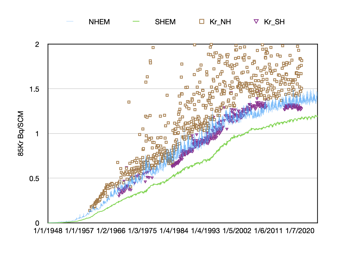

  
  

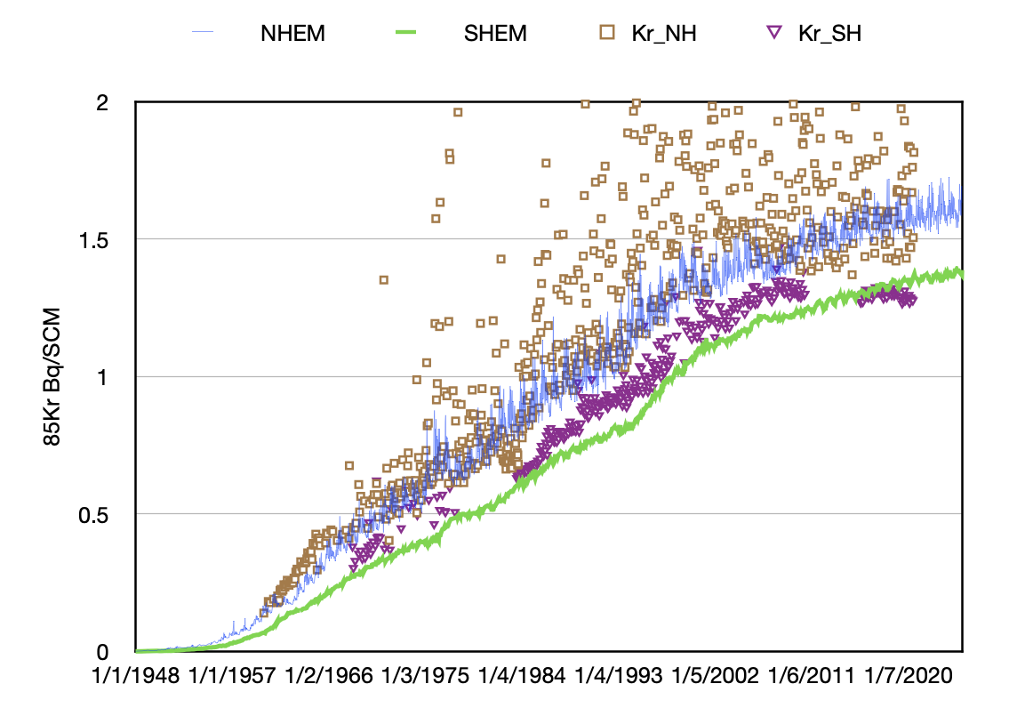
• The two model result graphics, the first, on the left, used the emissions as previously mentioned, and in the second, the emissions for all sources was increased by 15%. The model prediction curves, for hypothetical sampling locations in the remote Pacific Ocean, away from any nearby sources, should be closer to the baseline of the measurements, especially those in the southern hemisphere, because most of the krypton sources are located in the northern hemisphere. Not to discount any technical issues with the global dispersion model, but slight adjustments to the emissions are not unexpected given the uncertainty associated with most of the major sources and the difficulty obtaining accurate emission data.

As discussed in the paper¹, for any particular DATEM experimenal data set, the nearby sources are removed from the calculation, the baseline of the calculated concentrations are adjusted to give a best fit with the measurement minimums, and the remaining differences between the measurements and model predictions are assumed to be plumes from the source under evaluation. See the You Tube video to show how to compile, configure, and run the global model.